Building a Kenyan Portfolio You Can Explain and Maintain
Part 3 of 4: Allocation, diversification, risk budgets, and implementation
Selecting a good company answers only part of the investment question. The next decision is how much to own alongside everything else that matters to the household. An investor can understand several banks well and still accumulate a portfolio whose income, market value, and employment prospects all depend on the same credit cycle. Another can own companies from many sectors while remaining heavily exposed to government payments, local interest rates, and the shilling. Portfolio construction makes those connections visible. This article builds three educational allocations from a common research universe and tests the choices inside them. The accompanying workbook lets you change weights, expected returns, market relationships, costs, and purchase sizes. The purpose is to develop a portfolio whose structure follows an understandable plan and whose vulnerabilities can be examined before capital is committed.
Start with the investor's economic position outside the brokerage account. Salary, business income, property, pension savings, borrowing, and family commitments all influence the amount of investment risk the household can carry. A person whose income varies with construction activity already has a different exposure from someone receiving a stable pension. A planned payment in twelve months creates a different constraint from a retirement goal twenty years away. CFA Institute's asset-allocation framework places objectives and constraints at the beginning of the process [1]. For this exercise, the one-million-shilling portfolio is capital available after establishing an emergency reserve. That assumption makes the examples easier to compare. When adapting them, define the reserve and commitments first so that the investment allocation reflects the household's actual capacity to stay invested through changing conditions.
Translate that position into a short investment policy. State the portfolio's purpose, time horizon, cash needs, acceptable concentration, allowed instruments, and review process. Add the conditions under which the policy itself should change, such as a major income change, a new liability, or a shorter horizon. This document can be brief while still answering difficult questions. It tells the investor how to respond when a popular company becomes a large position, when a bill matures, or when an unexpected contribution arrives. It also separates a change in circumstances from a reaction to recent prices. The workbook turns several policy choices into editable constraints, including a single-equity limit, a bank-sector limit, and a minimum bill allocation. These controls make the intended structure visible throughout the calculations and implementation process.
Give each allocation a job
The three examples use the same seven equity names and a Treasury-bill sleeve so that the effect of allocation can be explored directly. The equity universe contains Equity Group, KCB, Co-operative Bank, Safaricom, BAT Kenya, Jubilee, and KenGen. These names provide business models for study across several sectors; the expected returns, volatilities, liquidity inputs, and entry prices are educational assumptions. Dated dividend observations appear separately in the screening workbook. Using a common universe means that differences between portfolios mainly reflect the amount committed to each exposure. It also makes comparisons easier to follow because the investor can inspect one set of company research notes and then decide how those cases should combine. Other researched companies can be substituted once their financial and market inputs have been assembled on a comparable basis.
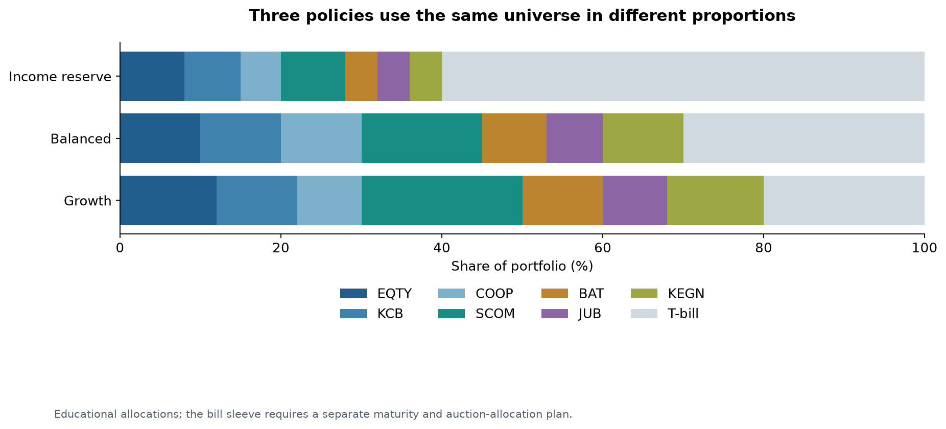
The Income Reserve allocation places 60% in the bill sleeve and 40% across equities. The equity weights are 8% Equity, 7% KCB, 5% Co-operative Bank, 8% Safaricom, and 4% each in BAT, Jubilee, and KenGen. This structure gives a substantial portion of capital a scheduled maturity while preserving participation in company earnings and distributions. Its role is to explore a portfolio with a smaller equity allocation and a relatively prominent cash-management function. The household would still organise actual bill purchases around its payment calendar and auction terms. The portfolio also retains sovereign and local purchasing-power exposure, which need explicit consideration. A useful evaluation asks whether its maturity schedule and income are aligned with the investor's needs, and whether the remaining equity risk is manageable during a period of weak business conditions.
The Balanced allocation places 30% in bills and 70% in equities. Equity, KCB, and Co-operative Bank each receive 10%; Safaricom receives 15%; BAT receives 8%; Jubilee receives 7%; and KenGen receives 10%. Banking therefore accounts for 30% of the whole portfolio, matching the teaching policy's sector ceiling. This allocation offers a useful central case because it creates meaningful exposure to several company models while retaining a bill sleeve for maturity management and future deployment. The label describes the example's intended role rather than a universal definition of balance. Its suitability for a real household depends on income stability, horizon, other assets, and the willingness to tolerate temporary and permanent losses. The workbook makes those trade-offs measurable through scenario returns, concentration checks, cash income, and risk-contribution calculations.
The Growth allocation reduces bills to 20% and raises equities to 80%. It holds 12% Equity, 10% KCB, 8% Co-operative Bank, 20% Safaricom, 10% BAT, 8% Jubilee, and 12% KenGen. The increased equity exposure creates more participation in the assumed company-return opportunities and more sensitivity to their joint outcomes. This can suit an educational exploration of longer-horizon accumulation where near-term spending is funded elsewhere. The investor should examine how a difficult early period would affect both the account and the ability to continue contributing. A larger equity allocation can be easier to sustain when the household understands the businesses, has a clear reserve, and follows a workable contribution policy. The allocation earns its place through those practical conditions and the tested outcomes, rather than through its name alone.
| Asset | Income Reserve | Balanced | Growth |
|---|---|---|---|
| Equity Group | 8% | 10% | 12% |
| KCB | 7% | 10% | 10% |
| Co-operative Bank | 5% | 10% | 8% |
| Safaricom | 8% | 15% | 20% |
| BAT Kenya | 4% | 8% | 10% |
| Jubilee | 4% | 7% | 8% |
| KenGen | 4% | 10% | 12% |
| Treasury-bill sleeve | 60% | 30% | 20% |
Understand what diversification is doing
Diversification depends on how holdings behave together. Markowitz's foundational portfolio research formalised the importance of those relationships when combining expected returns and risk [2]. In practical language, a holding can be valuable to a portfolio partly because its difficult periods occur differently from those of the other holdings. The workbook represents this through an explicit relationship matrix and derives the total portfolio risk from both individual variability and joint movements. Its initial relationships are assumptions generated from a common-factor model, giving a mathematically valid starting matrix. They are available for inspection and replacement with a carefully prepared historical estimate or a different scenario. This design allows the reader to see why adding another company can reduce, leave unchanged, or sometimes increase the portfolio's exposure to the outcomes that matter most.
Sector labels provide an initial map of concentration, but the deeper map follows economic exposures. Banks and insurers may both own government securities. An energy company may depend on an offtaker whose collections are sensitive to the wider economy. Consumer spending affects telecommunications, retail distribution, and loan repayment in different ways. Regional expansion can diversify domestic demand while adding currency, political, and operating risks. The investor can record these connections in a look-through exposure table and use them to design joint scenarios. This is particularly useful in a relatively concentrated local market because several apparently different holdings may respond to the same event. A portfolio can still make sense with these exposures, provided their scale is understood and the investor has considered how they interact with household income and commitments outside the account.
Company count is therefore only one part of diversification. Seven carefully researched shares can offer different business exposures, yet each position remains a meaningful ownership risk. Adding many very small positions can broaden exposure but increase the work required to understand and monitor them. Bessembinder's research on United States equities highlights the importance of a relatively small number of large long-term winners in aggregate wealth creation [3]. That evidence provides a useful reason to examine the trade-off between concentration and the opportunity to participate in exceptional outcomes. For this Kenyan exercise, it supports keeping the selection process open and evaluating the consequences of excluding businesses or sectors. The exact number of holdings should emerge from the opportunity set, research capacity, costs, and desired concentration rather than being treated as a complete measure of portfolio resilience.
The bill sleeve changes the portfolio's exposure in several ways. Holding a bill to maturity establishes a contractual receipt and reduces dependence on an equity sale for that portion of the plan. Repeated bill investment introduces uncertainty about future auction rates, while inflation changes the purchasing power of the proceeds. Sovereign credit and the investor's access to funds also remain relevant. In the risk workbook, the bill sleeve has a small assumed variability representing annual rollover-return uncertainty. It is therefore a modelling representation of a continuing allocation, while the bill-pricing workbook handles the cash flows of a specific security. Keeping those roles distinct helps the investor compare strategic allocation with actual maturity planning. The same distinction matters when replacing bills with longer bonds, whose market values respond differently to changes in required yields.
Estimate returns with visible assumptions
Expected equity return can be organised around starting income, growth in the underlying business, and the change in valuation between purchase and sale. This decomposition is useful even when the model ultimately uses an annual total-return assumption. It forces the investor to explain why the chosen return is plausible at the proposed price. A high dividend yield may be accompanied by limited growth, while a lower yield may accompany substantial reinvestment. A valuation multiple can expand, remain stable, or contract as the business and required returns change. The workbook's expected-return inputs are explicit teaching assumptions, making it easy to test a lower-return environment. Dated dividend observations inform the income calculation, but future total returns require a view about the business, its financing, and the price eventually realised for the ownership claim.
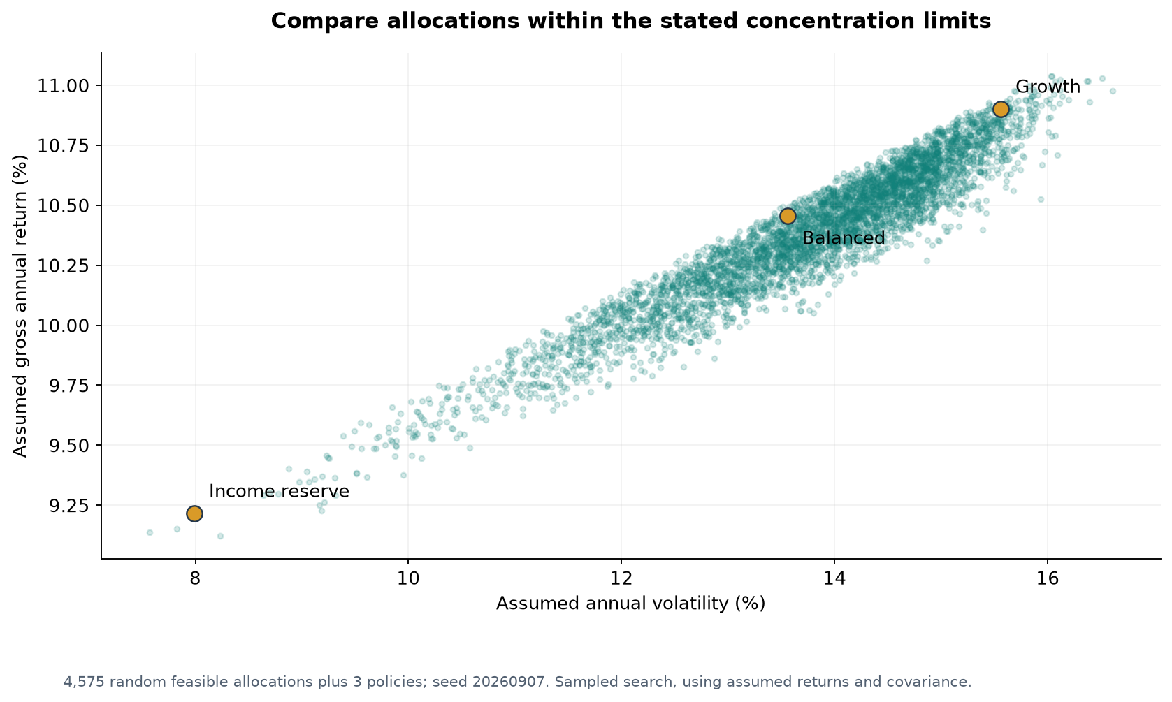
Equation (3.1), portfolio expected return = the sum of each allocation weight multiplied by its expected return, gives a simple calculation with a clear interpretation. Under the initial assumptions, the Income Reserve, Balanced, and Growth allocations produce annual expected returns of 9.215%, 10.455%, and 10.900% before the later implementation and dividend-tax adjustments. The comparison shows the reward assumed for increasing equity exposure within this particular universe. It also reveals how modest the difference can be relative to the additional uncertainty. The investor can lower the expected return of one holding, reduce all equity assumptions, or change the bill assumption and observe how the ranking moves. This is useful because it makes the allocation sensitive to the strength of the underlying investment cases rather than allowing an attractive portfolio label to determine the conclusion.
The corresponding assumed annual volatilities are approximately 7.99%, 13.56%, and 15.56%. Volatility describes variation around the modelled return pattern; it is one dimension of risk alongside cash shortfall, permanent business loss, and difficulties selling. The appendix shows how the matrix calculation produces these figures and how each holding contributes. In the main portfolio discussion, the practical question is whether the additional uncertainty helps advance the investor's goal enough to justify its consequences. A household with a near-term payment may care more about a dependable maturity than a higher expected return. A long-horizon investor with stable contributions may be able to tolerate greater variation. Comparing return and variability together makes those different priorities visible and helps explain why reasonable investors can choose different allocations from the same research universe.
Risk contribution adds another useful layer because an allocation's share of money can differ from its share of portfolio variability. A volatile holding that moves closely with several other positions can contribute substantial risk even at a moderate weight. A lower-volatility sleeve can hold a large amount of capital while contributing relatively little to the calculated market variation. The workbook provides each asset's contribution and checks that the contributions add to the portfolio total. The investor can then compare the result with the intended risk budget. If one business or sector dominates, the response might involve a smaller weight, a different holding, a larger bill sleeve, or simply a conscious acceptance of that exposure. The value of the calculation is that the choice becomes explicit and connected to the portfolio's behaviour.
Use optimisation as a comparison tool
Equal weighting is a useful benchmark because it is transparent and easy to maintain. A more elaborate allocation should explain what improves when weights depart from that starting point. DeMiguel, Garlappi, and Uppal found that estimation error challenged the out-of-sample performance of several optimisation approaches relative to a simple equal-weight rule in their datasets [4]. For this exercise, that finding encourages a practical comparison among simple policies, constrained alternatives, and the information required to support them. The investor can ask whether a small improvement in the model is worth additional concentration, trading, or sensitivity to uncertain inputs. This preserves the usefulness of optimisation while keeping the decision grounded in implementation. A portfolio with slightly weaker model statistics can still be attractive if its structure is easier to explain, monitor, and sustain.
The workbook includes a reproducible search across 4,578 feasible candidate allocations drawn from a seeded set of possible weights. The search applies the initial long-only, single-equity, banking, and bill constraints, then compares modelled risk and return. It identifies a lowest-variance candidate and a highest-Sharpe candidate within that sample. These are approximate search results whose exact weights depend on the inputs, constraints, and sampled candidates. The workbook preserves their weights and an audit sample, while the research script reproduces the wider calculation. This gives the reader a practical way to compare the three policy portfolios with alternatives. You can examine whether the selected candidate is economically sensible, whether the improvement is substantial, and which assumptions would need to be better supported before adopting a more finely tuned allocation.
Historical estimation offers another route, provided the input series is prepared carefully. Use consistent observation dates, adjusted prices, cash distributions, and corporate-action treatment. A thinly traded share can show unchanged prices on many days, making daily variability and cross-company relationships appear lower than the underlying economic exposure. Monthly observations may reduce some trading-frequency effects while providing fewer data points. The investor should record the sample period, missing observations, and the return convention before estimating a relationship matrix. Ledoit and Wolf's work on covariance shrinkage offers a method for stabilising noisy estimates by combining sample information with a structured target [5]. The appendix explains that idea and its mathematical equivalent. The practical objective is a relationship estimate that remains useful when the sample changes, rather than a matrix that only describes one historical window precisely.
Expected returns deserve at least as much sensitivity testing as historical relationships. A portfolio optimiser can concentrate heavily in a company whose expected return is only slightly overstated. One useful exercise lowers each equity assumption in turn and records how the preferred weights change. Another compares a common reduction in equity returns with a higher bill return. A third imposes stronger joint movements during stress. These exercises identify whether the proposed allocation depends on a broad business case or on a narrow numerical advantage. The investor can then place more weight on allocations that remain understandable across several plausible inputs. This approach also helps prioritise research: a company whose return assumption drives large allocation changes deserves close attention to valuation, earnings durability, and the evidence behind the expected return before its weight is increased materially.
Test combinations of problems
Scenario testing begins with an economic story and translates it into a consistent set of outcomes. The workbook includes a domestic credit shock, a shilling-and-inflation shock, an earnings recovery, and a liquidity shock. Each specifies one-year total returns across the holdings and the bill sleeve, then calculates the resulting portfolio return. The scenarios are assumed states rather than forecasts with assigned probabilities. Their purpose is to reveal how the allocation behaves when several positions move together. A credit shock, for example, can affect bank profits and valuations while also weakening customer spending and delaying payments elsewhere. The investor can adjust the severity and inspect the portfolio result. That makes the exercise useful even when precise event probabilities are unavailable, because it connects an understandable economic development with a measurable consequence for invested capital.
Dividend stress should also be considered jointly with price changes. A company facing weaker earnings may reduce its payout while its market value declines, affecting both current income and the amount available from a sale. The investor can test cuts across a sector and examine the cash-income calendar separately from total return. This is especially useful when distributions fund spending because a portfolio may remain solvent while producing less usable income than expected. The appropriate response can involve a larger reserve, a lower spending commitment, more diversification in income sources, or a different allocation. The workbook's separation of ordinary dividends, specials, and total returns makes these tests easier to follow. It also prevents the same dividend from being counted once as portfolio return and again as an additional source of wealth during compounding.
Liquidity stress asks what happens when the investor wants to trade at the same time as many other participants. A wider bid–ask spread, less available volume, or a delayed transaction can change the realised result. The position-sizing sheet estimates the days needed to acquire a position at an assumed fraction of daily traded value. For a sale, the same basic capacity question can be combined with a more conservative volume and price assumption. The investor can then decide whether a position should be built gradually or capped below its valuation-based allocation. This is a useful complement to market-volatility calculations because it concerns the process of changing ownership. A portfolio that looks well diversified on paper becomes more practical when the investor can explain how its holdings would be acquired, reduced, and converted into cash when needed.
Holding selection can also reflect the investor's values and restrictions. Tobacco, alcohol, particular financing practices, environmental exposures, or concentrated state ownership may sit outside a chosen mandate. The practical approach is to record the exclusion before comparing allocations, then rerun the construction process within the remaining universe. In this series, BAT is included as a financial-analysis example, and the same workbook can accommodate an alternative researched consumer business. An exclusion changes the available exposures and may affect income, diversification, and valuation opportunities. Those consequences can be explored directly rather than hidden inside a final portfolio weight. This makes the policy more coherent and easier to maintain because the investor knows which choices express a financial judgement, which express a personal constraint, and how the remaining holdings support the overall purpose of the portfolio.
A benchmark gives the allocation a useful reference for later evaluation. An investor might compare with a dated bill strategy, an appropriate broad equity total-return measure, or a fixed mix that reflects the policy's intended equity and bill exposure. The benchmark should use a compatible currency, cash-flow convention, and treatment of distributions and costs. A mixed portfolio will naturally behave differently from a pure equity price index, particularly when dividends and bill income are material. Establishing the benchmark before observing the result makes the subsequent comparison easier to interpret. The investor can then ask whether company selection, allocation, fees, or implementation explains the difference. This turns performance review into a learning process and helps distinguish a useful long-term policy from a short period in which a particular market exposure happened to perform strongly.
Convert weights into affordable orders
Equation (3.2), allocated cash = portfolio budget multiplied by target weight, begins the implementation. The number of shares then depends on the price, transaction costs, and allowed trading unit. The workbook rounds down to whole units and carries the residual as cash. For the Balanced example, the illustrative one-million-shilling budget produces KES 985,817 of securities and reserved bill cash, KES 13,716.34 of equity acquisition costs, and KES 466.66 of residual cash. These amounts reconcile to the original budget. The bill allocation is a cash reservation that must be converted into a specific face-value purchase using the bill calculator. This treatment gives the investor a feasible starting schedule and makes the difference between a target weight and an executable position visible before an order is placed.
Implementation also involves the custody and settlement process. The investor can verify an intermediary's licence and category through the CMA directory, then establish the account arrangements and applicable charges [6]. CDSC describes delivery-versus-payment settlement on a rolling T+3 cycle for the equity market [7]. Current broker instructions and corporate-action dates should accompany any actual order. The workbook's order quantities provide an educational plan, while the final limit price and available market quantity determine execution. Retain the contract note, charges, settlement details, and resulting holdings so that the portfolio record matches the account. This closes the loop between research, allocation, and ownership. It also creates a reliable starting point for later performance measurement, where a small difference in costs or share count can otherwise become difficult to explain.
Rebalancing keeps the portfolio aligned with its policy as prices and cash flows change. The investor can review on a schedule, respond when a weight moves outside a chosen band, or combine both approaches. New contributions and distributions can fund underweight positions before discretionary sales are considered. The choice depends on costs, liquidity, valuation, and the reason for the drift. A rising share price may reflect a stronger business, a richer valuation, or both, so a rebalance can be informed by the updated company case. CFA Institute's discussion of real-world allocation constraints highlights the role of liquidity and tax considerations in this process [8]. A clear rule makes the review repeatable while leaving room for judgement about whether the original policy and valuation assumptions still fit the investor's circumstances.
The completed portfolio should be explainable at three levels. At the household level, it supports a defined purpose and leaves essential commitments funded. At the company level, each equity has a business case, valuation range, and monitoring question. At the portfolio level, the weights reflect concentration limits, shared risks, liquidity, and implementation costs. The workbooks allow these levels to be changed and tested together, while the research notes preserve the reasoning behind the inputs. The final article follows the portfolio through time. It examines contributions, compounding, dividend cuts, changing inflation, withdrawals, and simulated market paths. That final stage turns the allocation from a one-time purchase plan into an ongoing process, showing how the investor can evaluate progress and adapt when the path differs from the assumptions used at the beginning.
Technical appendix and formula dictionary.
References
[1] CFA Institute, “Principles of Asset Allocation”. [Online]. Available: Source. Accessed: Sep. 7, 2026.
[2] H. Markowitz, “Portfolio Selection”, The Journal of Finance, vol. 7, no. 1, pp. 77–91, 1952, doi: 10.1111/j.1540-6261.1952.tb01525.x. [Online]. Available: Source. Accessed: Sep. 7, 2026.
[3] H. Bessembinder, “Do stocks outperform Treasury bills?”, Journal of Financial Economics, vol. 129, no. 3, pp. 440–457, 2018, doi: 10.1016/j.jfineco.2018.06.004. [Online]. Available: Source. Accessed: Sep. 7, 2026.
[4] V. DeMiguel, L. Garlappi, and R. Uppal, “Optimal Versus Naive Diversification: How Inefficient is the 1/N Portfolio Strategy?”, The Review of Financial Studies, vol. 22, no. 5, pp. 1915–1953, 2009, doi: 10.1093/rfs/hhm075. [Online]. Available: Source. Accessed: Sep. 7, 2026.
[5] O. Ledoit and M. Wolf, “Honey, I Shrunk the Sample Covariance Matrix”, The Journal of Portfolio Management, vol. 30, no. 4, pp. 110–119, 2004. [Online]. Available: Source. Accessed: Sep. 7, 2026.
[6] Capital Markets Authority, “Licensees directory”. [Online]. Available: Source. Accessed: Sep. 7, 2026.
[7] Central Depository and Settlement Corporation, “Depository, Clearing and Settlement”. [Online]. Available: Source. Accessed: Sep. 7, 2026.
[8] CFA Institute, “Asset Allocation with Real-World Constraints”. [Online]. Available: Source. Accessed: Sep. 7, 2026.
No public comments yet. The first thoughtful question can start the discussion.