Keeping a Kenyan Portfolio Useful as Life and Markets Change

Part 4 of 4: Compounding, scenarios, simulation, and portfolio management

A portfolio begins as a set of weights and becomes a sequence of decisions. Income arrives at different dates, companies change their distributions, markets move, and the household's ability to contribute can vary. A plan that looks attractive at the beginning needs a process for navigating those developments. This final article follows the educational portfolios through time using deterministic projections, scenario tests, and Monte Carlo simulations. The simulations create many possible paths from explicit assumptions, allowing the investor to examine a range of outcomes. The accompanying workbook also shows the annual cash-flow sequence in ordinary rows and columns. Together, these tools help connect the portfolio to its purpose: what the money might become, how much saving effort contributes, when spending could become difficult, and which adjustments make the plan more resilient.

Start by defining what success means at a particular date. A target of KES 3 million can refer to nominal shillings at that date or to the purchasing power of KES 3 million today. Those definitions lead to different required outcomes as prices change. The examples use a twenty-year horizon, KES 1 million of opening wealth, and KES 120,000 contributed at each year-end. The primary goal is KES 3 million in today's purchasing power. Contributions are held constant in nominal terms initially, so their real value declines when inflation is positive. These choices are editable and form the foundation of every comparison. Once they are visible, the investor can ask whether a different contribution path, longer horizon, lower spending target, or revised allocation offers the most practical improvement.

The annual order of events matters because money can earn a return only while it is invested. Equation (4.1), closing wealth = opening wealth grown by the net return plus contributions minus withdrawals, describes the teaching model's year-end sequence. A contribution made at the end of the year begins earning the following year's return. A withdrawal follows the year's investment result and contribution. The workbook records any amount that the available funds cannot meet, then floors invested wealth at zero. This makes the spending shortfall observable rather than allowing a negative account balance to imply unspecified borrowing. A monthly implementation can extend the same sequence to actual dates, but the annual version provides a clear starting point for understanding how return, saving, and spending interact over a long horizon.

Separate saving effort from investment performance

Compounding is the repeated application of returns to the capital that remains invested. With a constant return and no external cash flows, the calculation is simple. Adding contributions or withdrawals makes their timing part of the result. Equation (4.2), future value of opening capital = opening capital multiplied by the growth factor raised to the number of periods, describes the first component. The appendix adds the contribution series and works through the manual calculation. This is useful because the final account value combines both investment performance and the investor's saving effort. A larger ending balance can come from higher contributions even during mediocre markets. Separating those sources makes progress easier to evaluate and gives the household practical choices when the original investment assumptions turn out to be too optimistic or the saving capacity changes.

In the deterministic Balanced example, the assumed annual total return is 10.455% before equity-dividend withholding and implementation drag. The model subtracts a 0.3% annual implementation allowance and the withholding associated with the assumed recurring equity dividend yield. This gives a net annual return of approximately 9.8606% under the starting inputs. With KES 120,000 added at each year-end, the twenty-year result is approximately KES 13.324 million in nominal wealth. At constant 5% inflation, that is approximately KES 5.022 million in starting purchasing power. These calculations provide a transparent reference path. The investor can inspect every year and identify the contribution, investment gain, and inflation adjustment. The simulation then explores how varied returns and adverse episodes change the range around this smooth projection and the chance of reaching the chosen goal.

Dividend treatment needs consistency throughout that projection. A total-return assumption already includes the economic contribution of distributions, so reinvested dividends should remain within that return rather than being added again as a separate gain. Withholding reduces the portion retained by the investor, while implementation costs create a further deduction. If dividends fund household spending, the withdrawal schedule should record that cash leaving the portfolio. If they accumulate temporarily before reinvestment, the model can represent the delay and cash return separately. This treatment gives the investor a clear way to compare accumulation with income use. It also connects the first article's dividend analysis to the long-term projection: a lower ordinary payment can alter current cash availability and may accompany a different total-return outlook, depending on why the company has changed its distribution.

Inflation is applied through a cumulative price index. Equation (4.3), real wealth = nominal wealth divided by the cumulative price index, expresses the conversion into starting purchasing power. With constant 5% inflation over twenty years, the index is approximately 2.6533. A nominal balance must therefore be divided by that factor to describe what it can buy relative to the starting date. The workbook also allows separate inflation assumptions by year. This is useful when testing a period of elevated prices followed by a return to a lower rate. The investor can relate the general price assumption to the actual goal, since education, housing, health care, and other expenses may change differently. A goal-specific budget provides an additional check on whether the model's purchasing-power measure captures the commitment the portfolio is intended to support.

Test the assumptions before adding randomness

Scenario testing is the first step because it connects a set of assumptions with an understandable story. A lower-contribution case might represent a period of reduced income or a competing household commitment. A higher-inflation case might reflect a more expensive goal. An earnings shock can combine weaker company performance, lower dividends, and valuation pressure. Each case should change the inputs that create the outcome rather than applying an arbitrary haircut to the final wealth figure. The workbooks provide several starting scenarios and preserve the calculation sequence underneath them. This makes the results useful for planning. The investor can identify the cause of a shortfall and compare possible responses, such as a larger reserve, a different contribution schedule, a later target date, or a reduced dependence on selling equities during a difficult period.

Sensitivity analysis changes one input at a time to reveal where the plan is most exposed. In valuation, that might be the required return or terminal growth. In accumulation, it might be contributions, inflation, costs, or the investment horizon. In an income portfolio, it might be a sector-wide dividend cut. The useful output is a comparison that holds everything else consistent. The simulation experiments use the same underlying random draws when comparing several contribution and inflation cases, making the effect of the changed assumption easier to identify. This is especially helpful when two choices produce similar results because a fresh set of random paths could otherwise obscure the difference. The investor can then focus research and practical effort on the inputs that have the largest effect on the goal or the most realistic scope for improvement.

Sequence risk becomes important when money enters or leaves the account. Consider the same five annual returns arranged in opposite orders, with a withdrawal at each year-end. Losses early in the withdrawal period leave less capital available for the later recovery, while early gains can create a larger base before withdrawals reduce it. The workbook places these sequences side by side and shows the annual balances. The appendix works through the arithmetic manually. This exercise is useful for anyone moving from accumulation to spending because the average return alone leaves an important part of the experience unexplained. The household can respond through a maturity ladder, a spending reserve, flexible withdrawals, or a different allocation. Each response changes the timing relationship between the investment portfolio and the bills it needs to pay.

Use simulation to explore a range of paths

Monte Carlo simulation extends scenario analysis by generating many possible sequences from specified distributions and relationships. Glasserman's academic treatment provides the methodological foundation for simulation, reproducibility, and the distinction between numerical sampling error and uncertainty in the model itself [1]. In this series, the larger experiment runs 10,000 paths over twenty years for each allocation. It uses the asset return and variability assumptions from the construction exercise, with a shared market component that creates joint movements. Each path applies annual rebalancing, contribution timing, dividend-tax drag, and the implementation allowance. The results provide distributions of wealth and other outcomes rather than a single forecast. The investor can therefore examine the middle of the distribution, weaker outcomes, stronger outcomes, and the proportion of paths meeting the stated purchasing-power goal.

The return engine generates positive gross asset-return factors, which become ordinary returns after subtracting one. Its parameters are chosen to match the assumed arithmetic mean and volatility before the additional crisis regime. The technical appendix shows the transformation and the relationship between the shared normal shocks and asset returns. These are modelling choices with identifiable consequences. The engine does not use a fitted historical NSE return series, so its probabilities describe the stated educational assumptions. That makes it well suited to exploring how allocation, contributions, and adverse episodes interact. An investor developing a company-specific forecast can replace the assumptions and compare results. An investor building a historical model would first prepare a consistent total-return dataset and evaluate whether the chosen distribution and dependence structure adequately describe the risks relevant to the intended use.

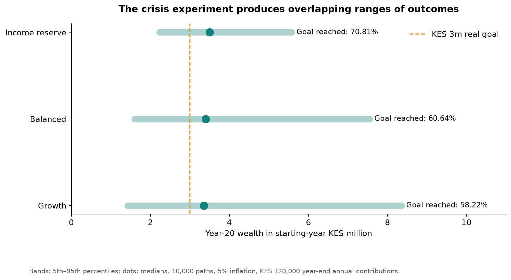
The crisis experiment adds an assumed 8% annual chance of a shared adverse episode. When it occurs, the equity gross-return factors receive additional proportional reductions, with losses varying by asset in the stated scenario. The bill sleeve receives no additional crisis haircut in this experiment, while its ordinary return remains variable. This creates a clear stress on equity-heavy allocations and changes the unconditional return distribution. The event probability is independent from year to year, making the mechanism simple to inspect. A more persistent crisis process could produce different results, and the appendix identifies that extension. The immediate value is practical: the investor can compare the same portfolio under a smooth return model and a model with explicit joint setbacks, then examine whether the plan remains useful when those setbacks arrive at inconvenient times.

The spreadsheet contains a separate 500-path aggregate-portfolio experiment whose formulas recalculate directly when its annual inputs change. It uses the Balanced portfolio's assumed mean and volatility and applies an additional 25% portfolio-level crisis reduction. The larger research engine models the eight assets separately and applies the asset-specific crisis assumptions. These two experiments answer related questions at different levels of detail, so their results are labelled separately. The spreadsheet is convenient for tracing individual years and testing a changed contribution or inflation path immediately. The larger engine supports comparisons across all three allocations with more simulation paths and richer dependence. This arrangement gives the reader both an accessible calculation surface and a reproducible extended analysis, with the assumptions for each kept visible in the workbook and technical appendix.

Read the results as conditional planning evidence

Under the larger engine's baseline assumptions, the Balanced allocation has a median twenty-year outcome of approximately KES 4.541 million in starting purchasing power. Its fifth-percentile outcome is approximately KES 2.236 million, and its ninety-fifth-percentile outcome is approximately KES 9.502 million. About 83.23% of paths reach the KES 3 million real goal. The spread is useful because it shows how different the experience can be despite a common allocation and saving schedule. The investor can compare the weaker outcomes with the minimum acceptable goal and the stronger outcomes with optional ambitions. This creates a more informative planning conversation than treating the median as the only meaningful result. It also highlights the role of flexibility: a plan with adjustable timing or spending can respond differently from one with a fixed amount required on a fixed date.

Adding the crisis regime changes the Balanced allocation's median real outcome to approximately KES 3.396 million. The fifth and ninety-fifth percentiles become approximately KES 1.602 million and KES 7.549 million, while the goal-success fraction becomes 60.64%. The mean real outcome is higher than the median because stronger paths pull the average upwards. These differences make the distribution shape relevant to the decision. A household focused on a minimum goal may place more weight on lower outcomes and shortfall probability than on the average wealth across all paths. The investor can now examine a concrete adjustment: contribute more, lower the goal, extend the horizon, or change the risk allocation. Each option can be tested against the same crisis assumptions, allowing its effect to be evaluated before a policy change is adopted.

The other allocations provide useful context for that result. In the crisis experiment, Income Reserve reaches the real goal in approximately 70.81% of paths, with median real wealth of approximately KES 3.498 million. Growth reaches it in approximately 58.22% of paths, with median real wealth of approximately KES 3.356 million. Growth also offers a wider upper range. Under these assumptions, the smaller equity allocation improves the chance of meeting this particular goal because the crisis losses affect the larger equity exposures more strongly. This is an informative result to investigate rather than a permanent ranking of investment styles. A different goal, return assumption, crisis structure, bill rate, or horizon can change the comparison. The value lies in seeing how the allocation serves a stated objective across the modelled distribution.

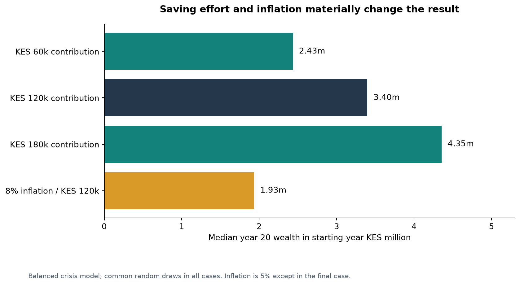
The contribution tests show another practical influence. In the Balanced crisis experiment, reducing annual contributions from KES 120,000 to KES 60,000 lowers the goal-success fraction to approximately 34.26%. Increasing them to KES 180,000 raises it to approximately 79.53%. The return paths are held consistent across these comparisons, so the change reflects saving effort under the same market conditions. This makes the result useful for household planning because contributions may be more directly influenced than market returns. The investor can explore a staged increase, occasional additional contributions, or a period of reduced saving followed by recovery. The annual-plan worksheet supports different amounts by year. The larger question is how to design a contribution routine that the household can sustain, especially when income and investment markets are under pressure at the same time.

Inflation sensitivity is equally important. Raising the assumed annual inflation rate from 5% to 8% in the Balanced crisis experiment reduces median real wealth to approximately KES 1.933 million and the goal-success fraction to approximately 18.16%. Nominal investment paths and contributions remain unchanged in this isolated test. The result shows the effect of a more demanding purchasing-power conversion, which is useful for understanding the exposure of a fixed nominal saving plan. In a broader economic scenario, returns, wages, contributions, and company earnings might also change with inflation. Those relationships can be added separately. Keeping this first sensitivity focused makes its meaning clear, then invites a more realistic second exercise: decide which cash flows are likely to adjust with prices and test how quickly those adjustments might occur for the household and its investments.

Measure risk along the path

Drawdown measures the decline from an earlier high. The simulation calculates it on a unitised investment path so that new contributions do not hide market losses. In the Balanced crisis experiment, the median maximum annual-observation drawdown is approximately 22.24%, and the ninety-fifth percentile is approximately 43.05%. These figures describe the largest peak-to-trough decline observed at the model's annual checkpoints. More frequent observations could reveal deeper interim falls. This matters because the investor experiences the journey as well as the ending balance. A plan that reaches its target in many paths may still require enduring periods of substantial loss. The household can compare that experience with its reserve, income stability, and willingness to continue investing, then adjust allocation or commitments if the path would be difficult to maintain.

Tail measures help examine the outcomes beyond a chosen percentile. Rockafellar and Uryasev's research develops conditional value-at-risk for general loss distributions [2]. The research engine reports the average of the worst 5% of terminal losses on the unitised investment path, alongside drawdown and goal shortfall. The loss is defined relative to the initial unit value, so a negative reported loss means that even the selected tail has an average gain over the full horizon. That convention is explained in the appendix to keep interpretation clear. The investor can choose a different loss definition, such as shortfall relative to a real goal, when that better matches the planning question. The central benefit is to examine the severity of adverse outcomes as well as how often a threshold is crossed in the experiment.

Withdrawal testing introduces a direct measure of spending failure. The extended experiment also starts with KES 1 million, makes no further contributions, and requests KES 100,000 at each year-end for twenty years. Under the Balanced crisis assumptions, approximately 59.04% of paths experience at least one withdrawal that available funds cannot fully meet. This is a materially different problem from accumulation, even though the asset-return assumptions are unchanged. The investor can test a lower withdrawal, a spending reserve, a different allocation, or a rule that adjusts withdrawals after weak years. The result gives the household a way to discuss sustainability in cash terms. It also connects the portfolio to the timing of actual commitments, where missing a payment can matter more than the average terminal value of the paths that remain well funded.

Sampling uncertainty tells the reader how precisely the simulation estimates its own conditional probability. For the 60.64% Balanced crisis success fraction across 10,000 paths, the estimated standard error is approximately 0.49 percentage points. A rough 95% sampling interval is therefore about one percentage point either side, using the usual normal approximation. The appendix shows the formula and substitution. This describes variation from using a finite number of paths under the same model. Changing expected returns, crisis frequency, inflation, or dependence can move the result much more. The practical approach is to report enough numerical precision to compare experiments while giving the assumptions equal prominence. Additional paths can stabilise the calculation, and additional research can improve the inputs; these are complementary ways of making the analysis more useful for a decision.

Keep the research and portfolio records connected

A regular portfolio review begins with information that can change the business case. New results, a distribution decision, a large acquisition, a change in financing, or a material operating development can alter the valuation and expected return. Update the relevant company fields, then examine the consequences for portfolio weight, income, and shared risk. Price changes also matter because they affect the valuation opportunity and current concentration. A useful review records both what changed and why the action follows. This keeps the process grounded in evidence rather than in the direction of the last price move. The monitoring worksheet provides space for the original thesis, new information, valuation changes, and resulting decision, allowing the investor to learn from the relationship between earlier expectations and the business outcomes that subsequently became observable.

Performance measurement then separates the quality of the investment result from the timing of contributions and withdrawals. A simple reconciliation compares ending wealth with opening wealth and net external flows to identify the currency amount of investment gain. A time-weighted return links subperiod results to evaluate the portfolio independently of the size of external flows. A money-weighted return incorporates the timing and amount of those flows to describe the investor's experience. The appendix explains the mathematical distinction and provides a dated example. The practical requirement is a reliable record of deposits, withdrawals, costs, distributions, and valuations. Once those records are consistent, the investor can compare with an appropriate benchmark and investigate whether company selection, allocation, fees, timing, or an accounting difference explains the gap between expectation and outcome.

Rebalancing and research updates work best as connected decisions. A holding can become overweight because its price has risen, because another holding has fallen, or because a contribution was allocated unevenly. The investor can first use available cash and new contributions to restore the intended structure where that remains attractive on valuation. A sale may be appropriate when concentration has become excessive or the business case has weakened. The transaction should then be evaluated using current liquidity and costs. The policy can specify review dates and allocation bands while retaining a record of justified exceptions. This makes the process both repeatable and adaptable. Over time, the investor gains a clearer understanding of which decisions improved the portfolio and which reflected assumptions that should be revised in the next round of research.

The research engine and workbook have different refresh boundaries, and the guide identifies them. Formula-driven spreadsheet outputs update when their linked inputs change. Seeded search candidates and the larger simulation report are reproducible snapshots that require rerunning the supplied research script after their assumptions are changed. The workbook includes a smaller live simulation for immediate exploration, while the full experiment preserves its seed, horizon, distributions, crisis assumptions, and cash-flow convention. This organisation gives the reader a practical way to maintain accuracy. Save the input version and resulting report together, then compare like with like when evaluating a revised policy. It also makes the analysis portable: another reader can follow the formulas, repeat the experiment, and see which differences arise from changed assumptions rather than from an undocumented calculation step.

The four-part process now forms a complete working cycle. Screening identifies the questions worth researching, financial analysis explains the business, valuation connects its prospects to price, and portfolio construction determines how the ownership cases fit together. Compounding and simulation then examine how that allocation interacts with saving, spending, inflation, and difficult markets over time. The useful outcome is a set of decisions you can explain and revisit. You know which figures came from a dated disclosure, which prices and returns are assumptions, how the models translate those inputs into results, and what evidence would justify a change. That is a practical foundation for ownership: a portfolio built around a purpose, supported by understandable calculations, and maintained through a research process that can grow more detailed as your knowledge and circumstances develop.

Technical appendix and formula dictionary.

References

[1] P. Glasserman, Monte Carlo Methods in Financial Engineering. New York, NY, USA: Springer, 2004, doi: 10.1007/978-0-387-21617-1. [Online]. Available: Publisher.

[2] R. T. Rockafellar and S. Uryasev, “Conditional value-at-risk for general loss distributions”, Journal of Banking & Finance, vol. 26, no. 7, pp. 1443–1471, 2002, doi: 10.1016/S0378-4266(02)00271-6. [Online]. Available: Source. Accessed: Sep. 7, 2026.